Support Vector Machines

In this lab, we use the sklearn.svm library to demonstrate the support vector classifier and the support vector machine.

We import some of our usual libraries.

import numpy as np
from matplotlib.pyplot import subplots, cm
import sklearn.model_selection as skm
from ISLP import load_data, confusion_table

We also collect the new imports needed for this lab.

from sklearn.svm import SVC
from ISLP.svm import plot as plot_svm
from sklearn.metrics import RocCurveDisplay

We will use the function RocCurveDisplay.from_estimator() to produce several ROC plots, using a shorthand roc_curve.

roc_curve = RocCurveDisplay.from_estimator # shorthand

Support Vector Classifier

We now use the SupportVectorClassifier() function (abbreviated SVC()) from sklearn to fit the support vector classifier for a given value of the parameter C. The C argument allows us to specify the cost of a violation to the margin. When the cost argument is small, then the margins will be wide and many support vectors will be on the margin or will violate the margin. When the C argument is large, then the margins will be narrow and there will be few support vectors on the margin or violating the margin.

Here we demonstrate the use of SVC() on a two-dimensional example, so that we can plot the resulting decision boundary. We begin by generating the observations, which belong to two classes, and checking whether the classes are linearly separable.

rng = np.random.default_rng(1)
X = rng.standard_normal((50, 2))
y = np.array([-1]*25+[1]*25)
X[y==1] += 1
fig, ax = subplots(figsize=(8,8))
ax.scatter(X[:,0],
           X[:,1],
           c=y,
           cmap=cm.coolwarm);

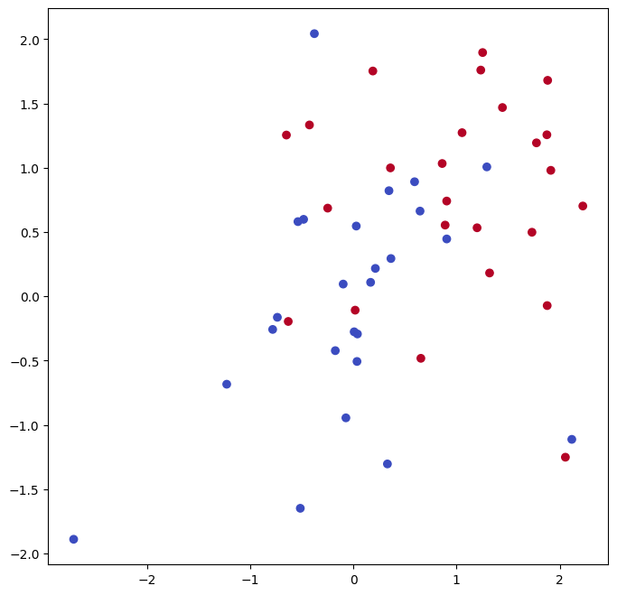
They are not. We now fit the classifier.

svm_linear = SVC(C=10, kernel='linear')
svm_linear.fit(X, y)

SVC(C=10, kernel='linear')

In a Jupyter environment, please rerun this cell to show the HTML representation or trust the notebook.
On GitHub, the HTML representation is unable to render, please try loading this page with nbviewer.org.

The support vector classifier with two features can be visualized by plotting values of its decision function. We have included a function for this in the ISLP package (inspired by a similar example in the sklearn docs).

fig, ax = subplots(figsize=(8,8))
plot_svm(X,
         y,
         svm_linear,
         ax=ax)

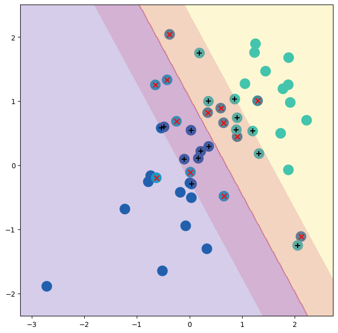
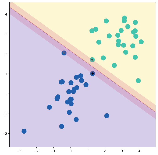
The decision boundary between the two classes is linear (because we used the argument kernel='linear'). The support vectors are marked with + and the remaining observations are plotted as circles.

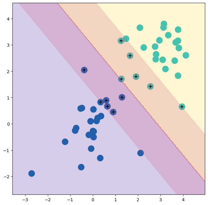
What if we instead used a smaller value of the cost parameter?

svm_linear_small = SVC(C=0.1, kernel='linear')
svm_linear_small.fit(X, y)
fig, ax = subplots(figsize=(8,8))
plot_svm(X,
         y,
         svm_linear_small,
         ax=ax)

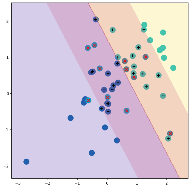
With a smaller value of the cost parameter, we obtain a larger number of support vectors, because the margin is now wider. For linear kernels, we can extract the coefficients of the linear decision boundary as follows:

svm_linear.coef_

array([[1.17303943, 0.77348227]])

Since the support vector machine is an estimator in sklearn, we can use the usual machinery to tune it.

kfold = skm.KFold(5, 
                  random_state=0,
                  shuffle=True)
grid = skm.GridSearchCV(svm_linear,
                        {'C':[0.001,0.01,0.1,1,5,10,100]},
                        refit=True,
                        cv=kfold,
                        scoring='accuracy')
grid.fit(X, y)
grid.best_params_

{'C': 1}

We can easily access the cross-validation errors for each of these models in grid.cv_results_. This prints out a lot of detail, so we extract the accuracy results only.

grid.cv_results_[('mean_test_score')]

array([0.46, 0.46, 0.72, 0.74, 0.74, 0.74, 0.74])

We see that C=1 results in the highest cross-validation accuracy of 0.74, though the accuracy is the same for several values of C. The classifier grid.best_estimator_ can be used to predict the class label on a set of test observations. Let’s generate a test data set.

X_test = rng.standard_normal((20, 2))
y_test = np.array([-1]*10+[1]*10)
X_test[y_test==1] += 1

Now we predict the class labels of these test observations. Here we use the best model selected by cross-validation in order to make the predictions.

best_ = grid.best_estimator_
y_test_hat = best_.predict(X_test)
confusion_table(y_test_hat, y_test)

Truth	-1	1
Predicted
-1	8	4
1	2	6

Thus, with this value of C, 70% of the test observations are correctly classified. What if we had instead used C=0.001?

svm_ = SVC(C=0.001,
           kernel='linear').fit(X, y)
y_test_hat = svm_.predict(X_test)
confusion_table(y_test_hat, y_test)

Truth	-1	1
Predicted
-1	2	0
1	8	10

In this case 60% of test observations are correctly classified.

We now consider a situation in which the two classes are linearly separable. Then we can find an optimal separating hyperplane using the SVC() estimator. We first further separate the two classes in our simulated data so that they are linearly separable:

X[y==1] += 1.9;
fig, ax = subplots(figsize=(8,8))
ax.scatter(X[:,0], X[:,1], c=y, cmap=cm.coolwarm);

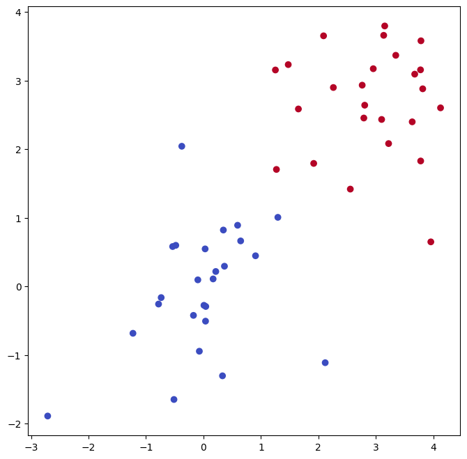
Now the observations are just barely linearly separable.

svm_ = SVC(C=1e5, kernel='linear').fit(X, y)
y_hat = svm_.predict(X)
confusion_table(y_hat, y)

Truth	-1	1
Predicted
-1	25	0
1	0	25

We fit the support vector classifier and plot the resulting hyperplane, using a very large value of C so that no observations are misclassified.

fig, ax = subplots(figsize=(8,8))
plot_svm(X,
         y,
         svm_,
         ax=ax)

Indeed no training errors were made and only three support vectors were used. In fact, the large value of C also means that these three support points are on the margin, and define it. One may wonder how good the classifier could be on test data that depends on only three data points! We now try a smaller value of C.

svm_ = SVC(C=0.1, kernel='linear').fit(X, y)
y_hat = svm_.predict(X)
confusion_table(y_hat, y)

Truth	-1	1
Predicted
-1	25	0
1	0	25

Using C=0.1, we again do not misclassify any training observations, but we also obtain a much wider margin and make use of twelve support vectors. These jointly define the orientation of the decision boundary, and since there are more of them, it is more stable. It seems possible that this model will perform better on test data than the model with C=1e5 (and indeed, a simple experiment with a large test set would bear this out).

fig, ax = subplots(figsize=(8,8))
plot_svm(X,
         y,
         svm_,
         ax=ax)

Support Vector Machine

In order to fit an SVM using a non-linear kernel, we once again use the SVC() estimator. However, now we use a different value of the parameter kernel. To fit an SVM with a polynomial kernel we use kernel="poly", and to fit an SVM with a radial kernel we use kernel="rbf". In the former case we also use the degree argument to specify a degree for the polynomial kernel (this is \(d\) in (9.22)), and in the latter case we use gamma to specify a value of \(\gamma\) for the radial basis kernel (9.24).

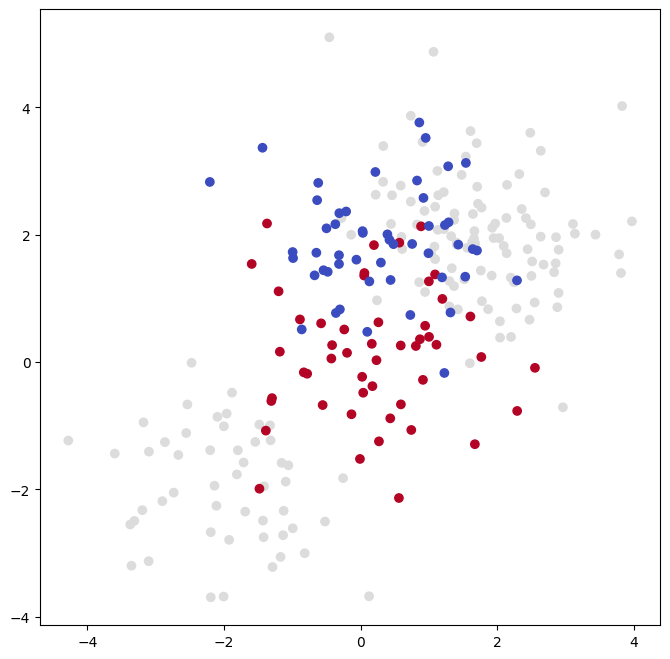
We first generate some data with a non-linear class boundary, as follows:

X = rng.standard_normal((200, 2))
X[:100] += 2
X[100:150] -= 2
y = np.array([1]*150+[2]*50)

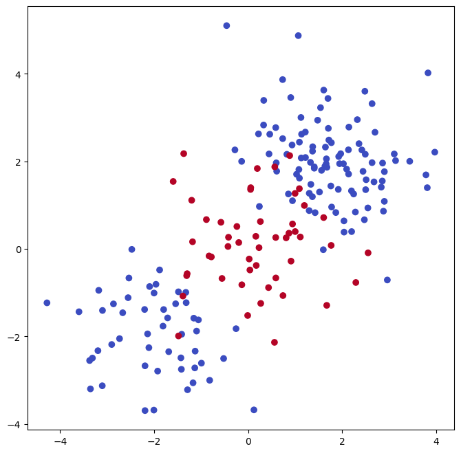
Plotting the data makes it clear that the class boundary is indeed non-linear.

fig, ax = subplots(figsize=(8,8))
ax.scatter(X[:,0],
           X[:,1],
           c=y,
           cmap=cm.coolwarm)

<matplotlib.collections.PathCollection at 0x282f53730>

The data is randomly split into training and testing groups. We then fit the training data using the SVC() estimator with a radial kernel and \(\gamma=1\):

(X_train, 
 X_test,
 y_train,
 y_test) = skm.train_test_split(X,
                                y,
                                test_size=0.5,
                                random_state=0)
svm_rbf = SVC(kernel="rbf", gamma=1, C=1)
svm_rbf.fit(X_train, y_train)

SVC(C=1, gamma=1)

In a Jupyter environment, please rerun this cell to show the HTML representation or trust the notebook.
On GitHub, the HTML representation is unable to render, please try loading this page with nbviewer.org.

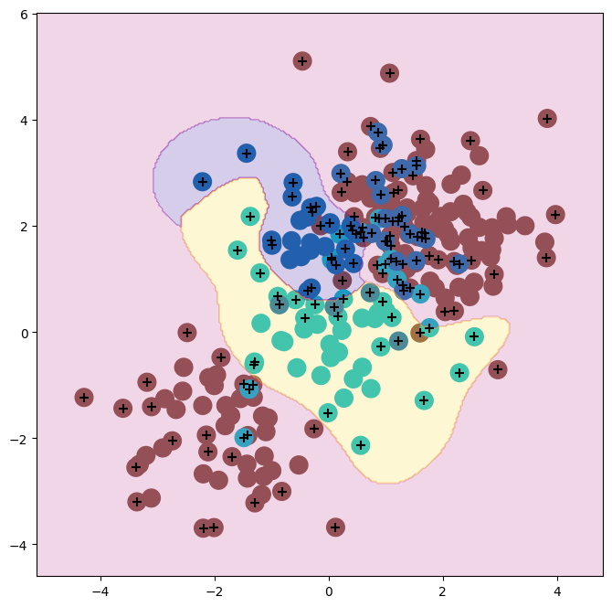
The plot shows that the resulting SVM has a decidedly non-linear boundary.

fig, ax = subplots(figsize=(8,8))
plot_svm(X_train,
         y_train,
         svm_rbf,
         ax=ax)

We can see from the figure that there are a fair number of training errors in this SVM fit. If we increase the value of C, we can reduce the number of training errors. However, this comes at the price of a more irregular decision boundary that seems to be at risk of overfitting the data.

svm_rbf = SVC(kernel="rbf", gamma=1, C=1e5)
svm_rbf.fit(X_train, y_train)
fig, ax = subplots(figsize=(8,8))
plot_svm(X_train,
         y_train,
         svm_rbf,
         ax=ax)

We can perform cross-validation using skm.GridSearchCV() to select the best choice of \(\gamma\) and C for an SVM with a radial kernel:

kfold = skm.KFold(5, 
                  random_state=0,
                  shuffle=True)
grid = skm.GridSearchCV(svm_rbf,
                        {'C':[0.1,1,10,100,1000],
                         'gamma':[0.5,1,2,3,4]},
                        refit=True,
                        cv=kfold,
                        scoring='accuracy');
grid.fit(X_train, y_train)
grid.best_params_

{'C': 1, 'gamma': 0.5}

The best choice of parameters under five-fold CV is achieved at C=1 and gamma=0.5, though several other values also achieve the same value.

best_svm = grid.best_estimator_
fig, ax = subplots(figsize=(8,8))
plot_svm(X_train,
         y_train,
         best_svm,
         ax=ax)

y_hat_test = best_svm.predict(X_test)
confusion_table(y_hat_test, y_test)

Truth	1	2
Predicted
1	69	6
2	6	19

With these parameters, 12% of test observations are misclassified by this SVM.

ROC Curves

SVMs and support vector classifiers output class labels for each observation. However, it is also possible to obtain fitted values for each observation, which are the numerical scores used to obtain the class labels. For instance, in the case of a support vector classifier, the fitted value for an observation $X= (X_1, X_2, \ldots, X_p)^T\( takes the form \)hat{beta}_0 + hat{beta}_1 X_1 + \hat{\beta}_2 X_2 + \ldots + \hat{\beta}_p X_p$. For an SVM with a non-linear kernel, the equation that yields the fitted value is given in (9.23). The sign of the fitted value determines on which side of the decision boundary the observation lies. Therefore, the relationship between the fitted value and the class prediction for a given observation is simple: if the fitted value exceeds zero then the observation is assigned to one class, and if it is less than zero then it is assigned to the other. By changing this threshold from zero to some positive value, we skew the classifications in favor of one class versus the other. By considering a range of these thresholds, positive and negative, we produce the ingredients for a ROC plot. We can access these values by calling the decision_function() method of a fitted SVM estimator.

The function ROCCurveDisplay.from_estimator() (which we have abbreviated to roc_curve()) will produce a plot of a ROC curve. It takes a fitted estimator as its first argument, followed by a model matrix \(X\) and labels \(y\). The argument name is used in the legend, while color is used for the color of the line. Results are plotted on our axis object ax.

fig, ax = subplots(figsize=(8,8))
roc_curve(best_svm,
          X_train,
          y_train,
          name='Training',
          color='r',
          ax=ax);

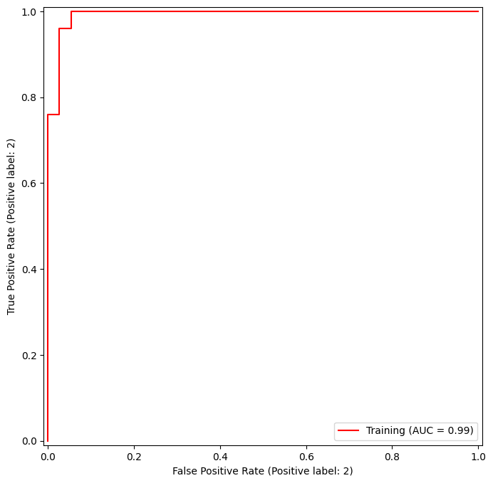
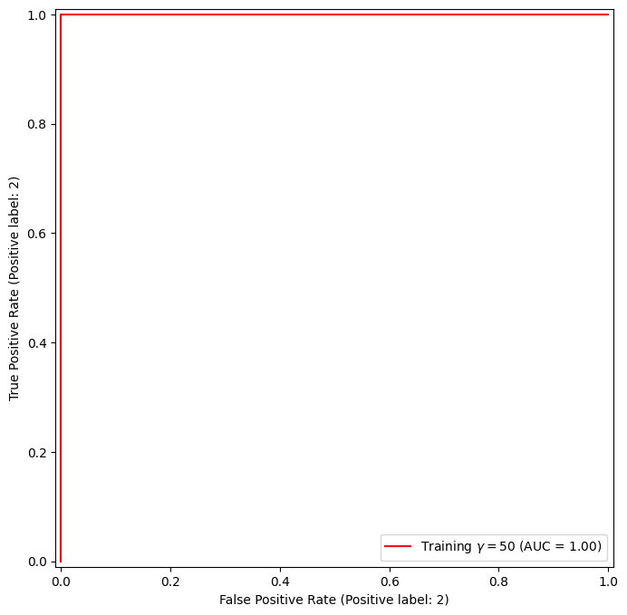
In this example, the SVM appears to provide accurate predictions. By increasing \(\gamma\) we can produce a more flexible fit and generate further improvements in accuracy.

svm_flex = SVC(kernel="rbf", 
              gamma=50,
              C=1)
svm_flex.fit(X_train, y_train)
fig, ax = subplots(figsize=(8,8))
roc_curve(svm_flex,
          X_train,
          y_train,
          name='Training $\gamma=50$',
          color='r',
          ax=ax);

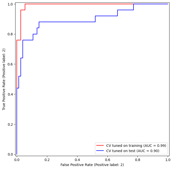
However, these ROC curves are all on the training data. We are really more interested in the level of prediction accuracy on the test data. When we compute the ROC curves on the test data, the model with \(\gamma=0.5\) appears to provide the most accurate results.

roc_curve(svm_flex,
          X_test,
          y_test,
          name='Test $\gamma=50$',
          color='b',
          ax=ax)
fig;

Let’s look at our tuned SVM.

fig, ax = subplots(figsize=(8,8))
for (X_, y_, c, name) in zip(
     (X_train, X_test),
     (y_train, y_test),
     ('r', 'b'),
     ('CV tuned on training',
      'CV tuned on test')):
    roc_curve(best_svm,
              X_,
              y_,
              name=name,
              ax=ax,
              color=c)

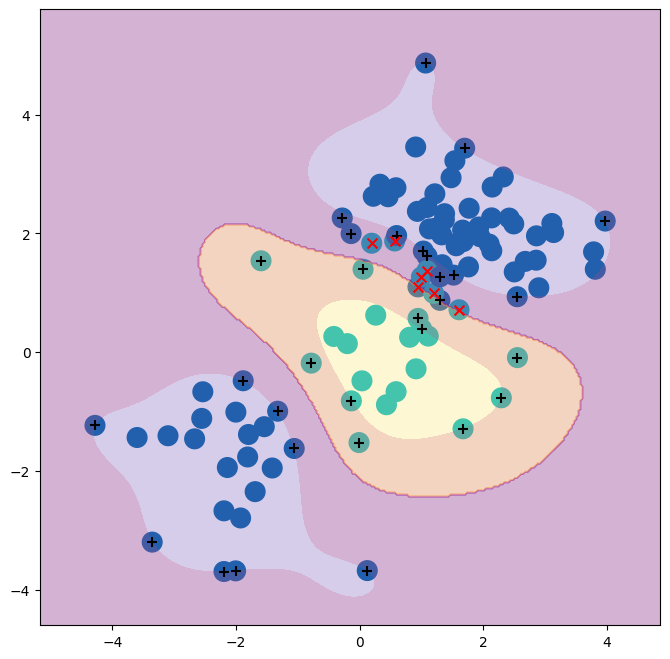
SVM with Multiple Classes

If the response is a factor containing more than two levels, then the SVC() function will perform multi-class classification using either the one-versus-one approach (when decision_function_shape=='ovo') or one-versus-rest {One-versus-rest is also known as one-versus-all.} (when decision_function_shape=='ovr'). We explore that setting briefly here by generating a third class of observations.

rng = np.random.default_rng(123)
X = np.vstack([X, rng.standard_normal((50, 2))])
y = np.hstack([y, [0]*50])
X[y==0,1] += 2
fig, ax = subplots(figsize=(8,8))
ax.scatter(X[:,0], X[:,1], c=y, cmap=cm.coolwarm);

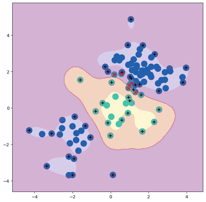
We now fit an SVM to the data:

svm_rbf_3 = SVC(kernel="rbf",
                C=10,
                gamma=1,
                decision_function_shape='ovo');
svm_rbf_3.fit(X, y)
fig, ax = subplots(figsize=(8,8))
plot_svm(X,
         y,
         svm_rbf_3,
         scatter_cmap=cm.tab10,
         ax=ax)

The sklearn.svm library can also be used to perform support vector regression with a numerical response using the estimator SupportVectorRegression().

Application to Gene Expression Data

We now examine the Khan data set, which consists of a number of tissue samples corresponding to four distinct types of small round blue cell tumors. For each tissue sample, gene expression measurements are available. The data set consists of training data, xtrain and ytrain, and testing data, xtest and ytest.

We examine the dimension of the data:

Khan = load_data('Khan')
Khan['xtrain'].shape, Khan['xtest'].shape

((63, 2308), (20, 2308))

This data set consists of expression measurements for 2,308 genes. The training and test sets consist of 63 and 20 observations, respectively.

We will use a support vector approach to predict cancer subtype using gene expression measurements. In this data set, there is a very large number of features relative to the number of observations. This suggests that we should use a linear kernel, because the additional flexibility that will result from using a polynomial or radial kernel is unnecessary.

khan_linear = SVC(kernel='linear', C=10)
khan_linear.fit(Khan['xtrain'], Khan['ytrain'])
confusion_table(khan_linear.predict(Khan['xtrain']),
                Khan['ytrain'])

Truth	1	2	3	4
Predicted
1	8	0	0	0
2	0	23	0	0
3	0	0	12	0
4	0	0	0	20

We see that there are no training errors. In fact, this is not surprising, because the large number of variables relative to the number of observations implies that it is easy to find hyperplanes that fully separate the classes. We are more interested in the support vector classifier’s performance on the test observations.

confusion_table(khan_linear.predict(Khan['xtest']),
                Khan['ytest'])

Truth	1	2	3	4
Predicted
1	3	0	0	0
2	0	6	2	0
3	0	0	4	0
4	0	0	0	5

We see that using C=10 yields two test set errors on these data.