Linear Models and Regularization Methods

In this lab we implement many of the techniques discussed in this chapter. We import some of our libraries at this top level.

Attention

Using skl.ElasticNet to fit ridge regression throws up many warnings. We have suppressed them below by a call to warnings.simplefilter().

import warnings
warnings.simplefilter("ignore")

import numpy as np
import pandas as pd
from matplotlib.pyplot import subplots
from statsmodels.api import OLS
import sklearn.model_selection as skm
import sklearn.linear_model as skl
from sklearn.preprocessing import StandardScaler
from ISLP import load_data
from ISLP.models import ModelSpec as MS
from functools import partial

We again collect the new imports needed for this lab. Readers will also have to have installed l0bnb using pip install l0bnb.

from sklearn.pipeline import Pipeline
from sklearn.decomposition import PCA
from sklearn.cross_decomposition import PLSRegression
from ISLP.models import \
     (Stepwise,
      sklearn_selected,
      sklearn_selection_path)
from l0bnb import fit_path

Subset Selection Methods

Here we implement methods that reduce the number of parameters in a model by restricting the model to a subset of the input variables.

Forward Selection

We will apply the forward-selection approach to the Hitters data. We wish to predict a baseball player’s Salary on the basis of various statistics associated with performance in the previous year.

First of all, we note that the Salary variable is missing for some of the players. The np.isnan() function can be used to identify the missing observations. It returns an array of the same shape as the input vector, with a True for any elements that are missing, and a False for non-missing elements. The sum() method can then be used to count all of the missing elements.

Hitters = load_data('Hitters')
np.isnan(Hitters['Salary']).sum()

59

We see that Salary is missing for 59 players. The dropna() method of data frames removes all of the rows that have missing values in any variable (by default — see Hitters.dropna?).

Hitters = Hitters.dropna();
Hitters.shape

(263, 20)

We first choose the best model using forward selection based on \(C_p\) (ref{Ch6:eq:cp}). This score is not built in as a metric to sklearn. We therefore define a function to compute it ourselves, and use it as a scorer. By default, sklearn tries to maximize a score, hence our scoring function computes the negative \(C_p\) statistic.

def nCp(sigma2, estimator, X, Y):
    "Negative Cp statistic"
    n, p = X.shape
    Yhat = estimator.predict(X)
    RSS = np.sum((Y - Yhat)**2)
    return -(RSS + 2 * p * sigma2) / n 

We need to estimate the residual variance \(\sigma^2\), which is the first argument in our scoring function above. We will fit the biggest model, using all the variables, and estimate \(\sigma^2\) based on its MSE.

design = MS(Hitters.columns.drop('Salary')).fit(Hitters)
Y = np.array(Hitters['Salary'])
X = design.transform(Hitters)
sigma2 = OLS(Y,X).fit().scale

The function sklearn_selected() expects a scorer with just three arguments — the last three in the definition of nCp() above. We use the function partial() first seen in Section~ref{Ch5-resample-lab:the-bootstrap} to freeze the first argument with our estimate of \(\sigma^2\).

neg_Cp = partial(nCp, sigma2)

We can now use neg_Cp() as a scorer for model selection.

Along with a score we need to specify the search strategy. This is done through the object Stepwise() in the ISLP.models package. The method Stepwise.first_peak() runs forward stepwise until any further additions to the model do not result in an improvement in the evaluation score. Similarly, the method Stepwise.fixed_steps() runs a fixed number of steps of stepwise search.

strategy = Stepwise.first_peak(design,
                               direction='forward',
                               max_terms=len(design.terms))

We now fit a linear regression model with Salary as outcome using forward selection. To do so, we use the function sklearn_selected() from the ISLP.models package. This takes a model from statsmodels along with a search strategy and selects a model with its fit method. Without specifying a scoring argument, the score defaults to MSE, and so all 19 variables will be selected.

hitters_MSE = sklearn_selected(OLS,
                               strategy)
hitters_MSE.fit(Hitters, Y)
hitters_MSE.selected_state_

('Assists',
 'AtBat',
 'CAtBat',
 'CHits',
 'CHmRun',
 'CRBI',
 'CRuns',
 'CWalks',
 'Division',
 'Errors',
 'Hits',
 'HmRun',
 'League',
 'NewLeague',
 'PutOuts',
 'RBI',
 'Runs',
 'Walks',
 'Years')

Using neg_Cp results in a smaller model, as expected, with just 10 variables selected.

hitters_Cp = sklearn_selected(OLS,
                               strategy,
                               scoring=neg_Cp)
hitters_Cp.fit(Hitters, Y)
hitters_Cp.selected_state_

('Assists',
 'AtBat',
 'CAtBat',
 'CRBI',
 'CRuns',
 'CWalks',
 'Division',
 'Hits',
 'PutOuts',
 'Walks')

Choosing Among Models Using the Validation Set Approach and Cross-Validation

As an alternative to using \(C_p\), we might try cross-validation to select a model in forward selection. For this, we need a method that stores the full path of models found in forward selection, and allows predictions for each of these. This can be done with the sklearn_selection_path() estimator from ISLP.models. The function cross_val_predict() from ISLP.models computes the cross-validated predictions for each of the models along the path, which we can use to evaluate the cross-validated MSE along the path.

Here we define a strategy that fits the full forward selection path. While there are various parameter choices for sklearn_selection_path(), we use the defaults here, which selects the model at each step based on the biggest reduction in RSS.

strategy = Stepwise.fixed_steps(design,
                                len(design.terms),
                                direction='forward')
full_path = sklearn_selection_path(OLS, strategy)

We now fit the full forward-selection path on the Hitters data and compute the fitted values.

full_path.fit(Hitters, Y)
Yhat_in = full_path.predict(Hitters)
Yhat_in.shape

(263, 20)

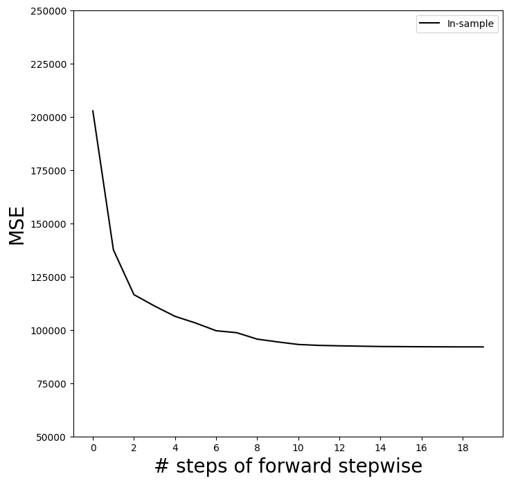
This gives us an array of fitted values — 20 steps in all, including the fitted mean for the null model — which we can use to evaluate in-sample MSE. As expected, the in-sample MSE improves each step we take, indicating we must use either the validation or cross-validation approach to select the number of steps. We fix the y-axis to range from 50,000 to 250,000 to compare to the cross-validation and validation set MSE below, as well as other methods such as ridge regression, lasso and principal components regression.

mse_fig, ax = subplots(figsize=(8,8))
insample_mse = ((Yhat_in - Y[:,None])**2).mean(0)
n_steps = insample_mse.shape[0]
ax.plot(np.arange(n_steps),
        insample_mse,
        'k', # color black
        label='In-sample')
ax.set_ylabel('MSE',
              fontsize=20)
ax.set_xlabel('# steps of forward stepwise',
              fontsize=20)
ax.set_xticks(np.arange(n_steps)[::2])
ax.legend()
ax.set_ylim([50000,250000]);

Notice the expression None in Y[:,None] above. This adds an axis (dimension) to the one-dimensional array Y, which allows it to be recycled when subtracted from the two-dimensional Yhat_in.

We are now ready to use cross-validation to estimate test error along the model path. We must use only the training observations to perform all aspects of model-fitting — including variable selection. Therefore, the determination of which model of a given size is best must be made using \emph{only the training observations} in each training fold. This point is subtle but important. If the full data set is used to select the best subset at each step, then the validation set errors and cross-validation errors that we obtain will not be accurate estimates of the test error.

We now compute the cross-validated predicted values using 5-fold cross-validation.

K = 5
kfold = skm.KFold(K,
                  random_state=0,
                  shuffle=True)
Yhat_cv = skm.cross_val_predict(full_path,
                                Hitters,
                                Y,
                                cv=kfold)
Yhat_cv.shape

(263, 20)

skm.cross_val_predict() The prediction matrix Yhat_cv is the same shape as Yhat_in; the difference is that the predictions in each row, corresponding to a particular sample index, were made from models fit on a training fold that did not include that row.

At each model along the path, we compute the MSE in each of the cross-validation folds. These we will average to get the mean MSE, and can also use the individual values to compute a crude estimate of the standard error of the mean. {The estimate is crude because the five error estimates are based on overlapping training sets, and hence are not independent.} Hence we must know the test indices for each cross-validation split. This can be found by using the split() method of kfold. Because we fixed the random state above, whenever we split any array with the same number of rows as \(Y\) we recover the same training and test indices, though we simply ignore the training indices below.

cv_mse = []
for train_idx, test_idx in kfold.split(Y):
    errors = (Yhat_cv[test_idx] - Y[test_idx,None])**2
    cv_mse.append(errors.mean(0)) # column means
cv_mse = np.array(cv_mse).T
cv_mse.shape

(20, 5)

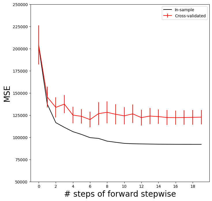
We now add the cross-validation error estimates to our MSE plot. We include the mean error across the five folds, and the estimate of the standard error of the mean.

ax.errorbar(np.arange(n_steps), 
            cv_mse.mean(1),
            cv_mse.std(1) / np.sqrt(K),
            label='Cross-validated',
            c='r') # color red
ax.set_ylim([50000,250000])
ax.legend()
mse_fig

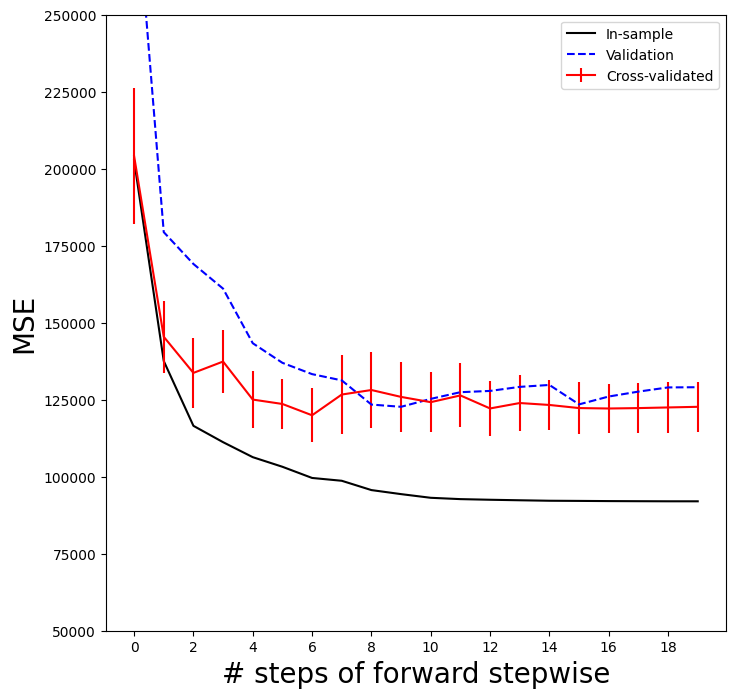
To repeat the above using the validation set approach, we simply change our cv argument to a validation set: one random split of the data into a test and training. We choose a test size of 20%, similar to the size of each test set in 5-fold cross-validation.skm.ShuffleSplit()

validation = skm.ShuffleSplit(n_splits=1, 
                              test_size=0.2,
                              random_state=0)
for train_idx, test_idx in validation.split(Y):
    full_path.fit(Hitters.iloc[train_idx],
                  Y[train_idx])
    Yhat_val = full_path.predict(Hitters.iloc[test_idx])
    errors = (Yhat_val - Y[test_idx,None])**2
    validation_mse = errors.mean(0)

As for the in-sample MSE case, the validation set approach does not provide standard errors.

ax.plot(np.arange(n_steps), 
        validation_mse,
        'b--', # color blue, broken line
        label='Validation')
ax.set_xticks(np.arange(n_steps)[::2])
ax.set_ylim([50000,250000])
ax.legend()
mse_fig

Best Subset Selection

Forward stepwise is a greedy selection procedure; at each step it augments the current set by including one additional variable. We now apply best subset selection to the Hitters data, which for every subset size, searches for the best set of predictors.

We will use a package called l0bnb to perform best subset selection. Instead of constraining the subset to be a given size, this package produces a path of solutions using the subset size as a penalty rather than a constraint. Although the distinction is subtle, the difference comes when we cross-validate.

D = design.fit_transform(Hitters)
D = D.drop('intercept', axis=1)
X = np.asarray(D)

Here we excluded the first column corresponding to the intercept, as l0bnb will fit the intercept separately. We can find a path using the fit_path() function.

path = fit_path(X, 
                Y,
                max_nonzeros=X.shape[1])

Preprocessing Data.
BnB Started.

Iteration: 1. Number of non-zeros:  1
Iteration: 2. Number of non-zeros:  2

Iteration: 3. Number of non-zeros:  2

Iteration: 4. Number of non-zeros:  2

Iteration: 5. Number of non-zeros:  3

Iteration: 6. Number of non-zeros:  3

Iteration: 7. Number of non-zeros:  4

Iteration: 8. Number of non-zeros:  9
Iteration: 9. Number of non-zeros:  9
Iteration: 10. Number of non-zeros:  9
Iteration: 11. Number of non-zeros:  9
Iteration: 12. Number of non-zeros:  9
Iteration: 13. Number of non-zeros:  9
Iteration: 14. Number of non-zeros:  9
Iteration: 15. Number of non-zeros:  9
Iteration: 16. Number of non-zeros:  9
Iteration: 17. Number of non-zeros:  9
Iteration: 18. Number of non-zeros:  17
Iteration: 19. Number of non-zeros:  19

The function fit_path() returns a list whose values include the fitted coefficients as B, an intercept as B0, as well as a few other attributes related to the particular path algorithm used. Such details are beyond the scope of this book.

path[3]

{'B': array([0.        , 3.25484367, 0.        , 0.        , 0.        ,
        0.        , 0.        , 0.        , 0.        , 0.        ,
        0.        , 0.67775265, 0.        , 0.        , 0.        ,
        0.        , 0.        , 0.        , 0.        ]),
 'B0': -38.98216739555505,
 'lambda_0': 0.011416248027450187,
 'M': 0.5829861733382012,
 'Time_exceeded': False}

In the example above, we see that at the fourth step in the path, we have two nonzero coefficients in 'B', corresponding to the value \(0.114\) for the penalty parameter lambda_0. We could make predictions using this sequence of fits on a validation set as a function of lambda_0, or with more work using cross-validation.

Ridge Regression and the Lasso

We will use the sklearn.linear_model package (for which we use skl as shorthand below) to fit ridge and lasso regularized linear models on the Hitters data. We start with the model matrix X (without an intercept) that we computed in the previous section on best subset regression.

Ridge Regression

We will use the function skl.ElasticNet() to fit both ridge and the lasso. To fit a path of ridge regressions models, we use skl.ElasticNet.path(), which can fit both ridge and lasso, as well as a hybrid mixture; ridge regression corresponds to l1_ratio=0. It is good practice to standardize the columns of X in these applications, if the variables are measured in different units. Since skl.ElasticNet() does no normalization, we have to take care of that ourselves. Since we standardize first, in order to find coefficient estimates on the original scale, we must unstandardize the coefficient estimates. The parameter \(\lambda\) in (ref{Ch6:ridge}) and (ref{Ch6:LASSO}) is called alphas in sklearn. In order to be consistent with the rest of this chapter, we use lambdas rather than alphas in what follows. {At the time of publication, ridge fits like the one in code chunk [22] issue unwarranted convergence warning messages; we expect these to disappear as this package matures.}

Xs = X - X.mean(0)[None,:]
X_scale = X.std(0)
Xs = Xs / X_scale[None,:]
lambdas = 10**np.linspace(8, -2, 100) / Y.std()
soln_array = skl.ElasticNet.path(Xs,
                                 Y,
                                 l1_ratio=0.,
                                 alphas=lambdas)[1]
soln_array.shape

(19, 100)

Here we extract the array of coefficients corresponding to the solutions along the regularization path. By default the skl.ElasticNet.path method fits a path along an automatically selected range of \(\lambda\) values, except for the case when l1_ratio=0, which results in ridge regression (as is the case here). {The reason is rather technical; for all models except ridge, we can find the smallest value of $\lambda$ for which all coefficients are zero. For ridge this value is $\infty$.} So here we have chosen to implement the function over a grid of values ranging from \(\lambda=10^{8}\) to \(\lambda=10^{-2}\) scaled by the standard deviation of \(y\), essentially covering the full range of scenarios from the null model containing only the intercept, to the least squares fit.

Associated with each value of \(\lambda\) is a vector of ridge regression coefficients, that can be accessed by a column of soln_array. In this case, soln_array is a \(19 \times 100\) matrix, with 19 rows (one for each predictor) and 100 columns (one for each value of \(\lambda\)).

We transpose this matrix and turn it into a data frame to facilitate viewing and plotting.

soln_path = pd.DataFrame(soln_array.T,
                         columns=D.columns,
                         index=-np.log(lambdas))
soln_path.index.name = 'negative log(lambda)'
soln_path

	AtBat	Hits	HmRun	Runs	RBI	Walks	Years	CAtBat	CHits	CHmRun	CRuns	CRBI	CWalks	League[N]	Division[W]	PutOuts	Assists	Errors	NewLeague[N]
negative log(lambda)
-12.310855	0.000800	0.000889	0.000695	0.000851	0.000911	0.000900	0.000812	0.001067	0.001113	0.001064	0.001141	0.001149	0.000993	-0.000029	-0.000390	0.000609	0.000052	-0.000011	-0.000006
-12.078271	0.001010	0.001122	0.000878	0.001074	0.001150	0.001135	0.001025	0.001346	0.001404	0.001343	0.001439	0.001450	0.001253	-0.000037	-0.000492	0.000769	0.000065	-0.000014	-0.000007
-11.845686	0.001274	0.001416	0.001107	0.001355	0.001451	0.001433	0.001293	0.001698	0.001772	0.001694	0.001816	0.001830	0.001581	-0.000046	-0.000621	0.000970	0.000082	-0.000017	-0.000009
-11.613102	0.001608	0.001787	0.001397	0.001710	0.001831	0.001808	0.001632	0.002143	0.002236	0.002138	0.002292	0.002309	0.001995	-0.000058	-0.000784	0.001224	0.000104	-0.000022	-0.000012
-11.380518	0.002029	0.002255	0.001763	0.002158	0.002310	0.002281	0.002059	0.002704	0.002821	0.002698	0.002892	0.002914	0.002517	-0.000073	-0.000990	0.001544	0.000131	-0.000028	-0.000015
...	...	...	...	...	...	...	...	...	...	...	...	...	...	...	...	...	...	...	...
9.784658	-290.823989	336.929968	37.322686	-59.748520	-26.507086	134.855915	-17.216195	-387.775826	89.573601	-12.273926	476.079273	257.271255	-213.124780	31.258215	-58.457857	78.761266	53.622113	-22.208456	-12.402891
10.017243	-290.879272	337.113713	37.431373	-59.916820	-26.606957	134.900549	-17.108041	-388.458404	89.000707	-12.661459	477.031349	257.966790	-213.280891	31.256434	-58.448850	78.761240	53.645147	-22.198802	-12.391969
10.249827	-290.923382	337.260446	37.518064	-60.051166	-26.686604	134.936136	-17.022194	-388.997470	88.537380	-12.971603	477.791860	258.523025	-213.405740	31.254958	-58.441682	78.761230	53.663357	-22.191071	-12.383205
10.482412	-290.958537	337.377455	37.587122	-60.158256	-26.750044	134.964477	-16.954081	-389.423414	88.164178	-13.219329	478.398404	258.967059	-213.505412	31.253747	-58.435983	78.761230	53.677759	-22.184893	-12.376191
10.714996	-290.986528	337.470648	37.642077	-60.243522	-26.800522	134.987027	-16.900054	-389.760135	87.864551	-13.416889	478.881540	259.321007	-213.584869	31.252760	-58.431454	78.761235	53.689152	-22.179964	-12.370587

100 rows × 19 columns

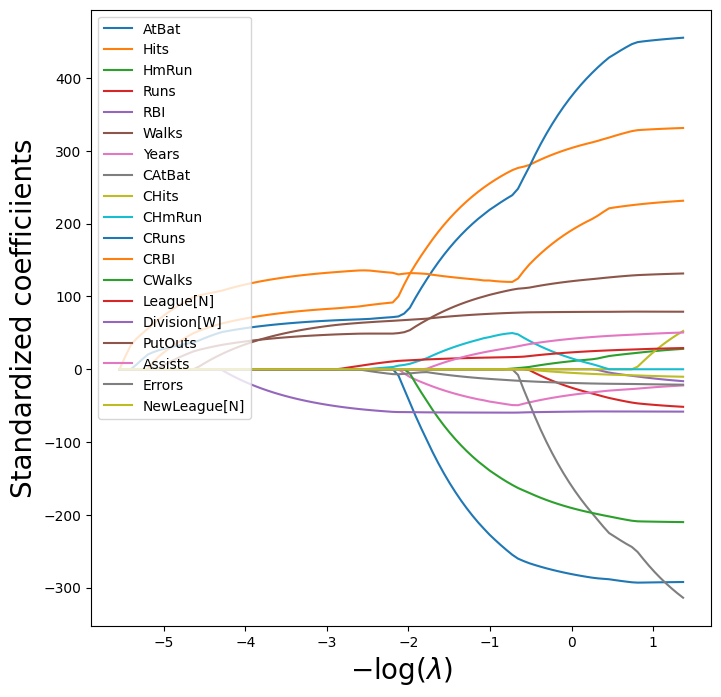
We plot the paths to get a sense of how the coefficients vary with \(\lambda\). To control the location of the legend we first set legend to False in the plot method, adding it afterward with the legend() method of ax.

path_fig, ax = subplots(figsize=(8,8))
soln_path.plot(ax=ax, legend=False)
ax.set_xlabel('$-\log(\lambda)$', fontsize=20)
ax.set_ylabel('Standardized coefficients', fontsize=20)
ax.legend(loc='upper left');

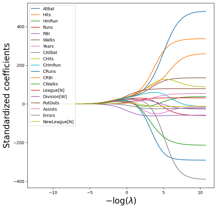
(We have used latex formatting in the horizontal label, in order to format the Greek \(\lambda\) appropriately.) We expect the coefficient estimates to be much smaller, in terms of \(\ell_2\) norm, when a large value of \(\lambda\) is used, as compared to when a small value of \(\lambda\) is used. (Recall that the \(\ell_2\) norm is the square root of the sum of squared coefficient values.) We display the coefficients at the \(40\)th step, where \(\lambda\) is 25.535.

beta_hat = soln_path.loc[soln_path.index[39]]
lambdas[39], beta_hat

(25.53538897200662,
 AtBat           5.433750
 Hits            6.223582
 HmRun           4.585498
 Runs            5.880855
 RBI             6.195921
 Walks           6.277975
 Years           5.299767
 CAtBat          7.147501
 CHits           7.539495
 CHmRun          7.182344
 CRuns           7.728649
 CRBI            7.790702
 CWalks          6.592901
 League[N]       0.042445
 Division[W]    -3.107159
 PutOuts         4.605263
 Assists         0.378371
 Errors         -0.135196
 NewLeague[N]    0.150323
 Name: -3.240065292879872, dtype: float64)

Let’s compute the \(\ell_2\) norm of the standardized coefficients.

np.linalg.norm(beta_hat)

24.17061720144378

In contrast, here is the \(\ell_2\) norm when \(\lambda\) is 2.44e-01. Note the much larger \(\ell_2\) norm of the coefficients associated with this smaller value of \(\lambda\).

beta_hat = soln_path.loc[soln_path.index[59]]
lambdas[59], np.linalg.norm(beta_hat)

(0.24374766133488554, 160.42371017725912)

Above we normalized X upfront, and fit the ridge model using Xs. The Pipeline() object in sklearn provides a clear way to separate feature normalization from the fitting of the ridge model itself.

ridge = skl.ElasticNet(alpha=lambdas[59], l1_ratio=0)
scaler = StandardScaler(with_mean=True,  with_std=True)
pipe = Pipeline(steps=[('scaler', scaler), ('ridge', ridge)])
pipe.fit(X, Y)

Pipeline(steps=[('scaler', StandardScaler()),
                ('ridge', ElasticNet(alpha=0.24374766133488554, l1_ratio=0))])

In a Jupyter environment, please rerun this cell to show the HTML representation or trust the notebook.
On GitHub, the HTML representation is unable to render, please try loading this page with nbviewer.org.

We show that it gives the same \(\ell_2\) norm as in our previous fit on the standardized data.

np.linalg.norm(ridge.coef_)

160.42371017725904

Notice that the operation pipe.fit(X, Y) above has changed the ridge object, and in particular has added attributes such as coef_ that were not there before.

Estimating Test Error of Ridge Regression

Choosing an a priori value of \(\lambda\) for ridge regression is difficult if not impossible. We will want to use the validation method or cross-validation to select the tuning parameter. The reader may not be surprised that the Pipeline() approach can be used in skm.cross_validate() with either a validation method (i.e. validation) or \(k\)-fold cross-validation.

We fix the random state of the splitter so that the results obtained will be reproducible.

validation = skm.ShuffleSplit(n_splits=1,
                              test_size=0.5,
                              random_state=0)
ridge.alpha = 0.01
results = skm.cross_validate(ridge,
                             X,
                             Y,
                             scoring='neg_mean_squared_error',
                             cv=validation)
-results['test_score']

array([134214.00419204])

The test MSE is 1.342e+05. Note that if we had instead simply fit a model with just an intercept, we would have predicted each test observation using the mean of the training observations. We can get the same result by fitting a ridge regression model with a very large value of \(\lambda\). Note that 1e10 means \(10^{10}\).

ridge.alpha = 1e10
results = skm.cross_validate(ridge,
                             X,
                             Y,
                             scoring='neg_mean_squared_error',
                             cv=validation)
-results['test_score']

array([231788.32155285])

Obviously choosing \(\lambda=0.01\) is arbitrary, so we will use cross-validation or the validation-set approach to choose the tuning parameter \(\lambda\). The object GridSearchCV() allows exhaustive grid search to choose such a parameter.

We first use the validation set method to choose \(\lambda\).

param_grid = {'ridge__alpha': lambdas}
grid = skm.GridSearchCV(pipe,
                        param_grid,
                        cv=validation,
                        scoring='neg_mean_squared_error')
grid.fit(X, Y)
grid.best_params_['ridge__alpha']
grid.best_estimator_

Pipeline(steps=[('scaler', StandardScaler()),
                ('ridge', ElasticNet(alpha=0.005899006046740856, l1_ratio=0))])

In a Jupyter environment, please rerun this cell to show the HTML representation or trust the notebook.
On GitHub, the HTML representation is unable to render, please try loading this page with nbviewer.org.

Alternatively, we can use 5-fold cross-validation.

grid = skm.GridSearchCV(pipe, 
                        param_grid,
                        cv=kfold,
                        scoring='neg_mean_squared_error')
grid.fit(X, Y)
grid.best_params_['ridge__alpha']
grid.best_estimator_

Pipeline(steps=[('scaler', StandardScaler()),
                ('ridge', ElasticNet(alpha=0.01185247763144249, l1_ratio=0))])

In a Jupyter environment, please rerun this cell to show the HTML representation or trust the notebook.
On GitHub, the HTML representation is unable to render, please try loading this page with nbviewer.org.

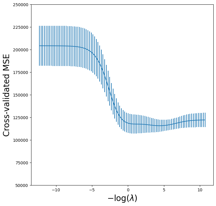
Recall we set up the kfold object for 5-fold cross-validation on page~pageref{line:choos-among-models}. We now plot the cross-validated MSE as a function of \(-\log(\lambda)\), which has shrinkage decreasing from left to right.

ridge_fig, ax = subplots(figsize=(8,8))
ax.errorbar(-np.log(lambdas),
            -grid.cv_results_['mean_test_score'],
            yerr=grid.cv_results_['std_test_score'] / np.sqrt(K))
ax.set_ylim([50000,250000])
ax.set_xlabel('$-\log(\lambda)$', fontsize=20)
ax.set_ylabel('Cross-validated MSE', fontsize=20);

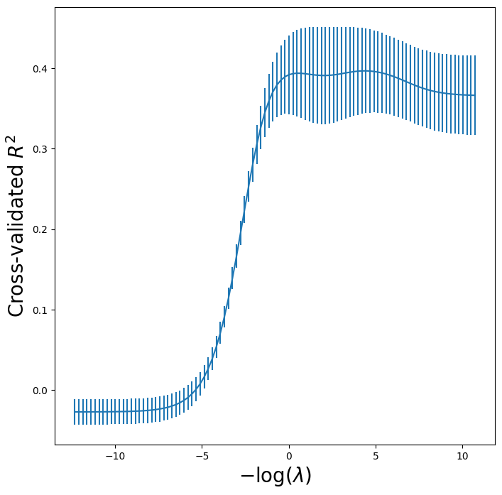
One can cross-validate different metrics to choose a parameter. The default metric for skl.ElasticNet() is test \(R^2\). Let’s compare \(R^2\) to MSE for cross-validation here.

grid_r2 = skm.GridSearchCV(pipe, 
                           param_grid,
                           cv=kfold)
grid_r2.fit(X, Y)

GridSearchCV(cv=KFold(n_splits=5, random_state=0, shuffle=True),
             estimator=Pipeline(steps=[('scaler', StandardScaler()),
                                       ('ridge',
                                        ElasticNet(alpha=10000000000.0,
                                                   l1_ratio=0))]),
             param_grid={'ridge__alpha': array([2.22093791e+05, 1.76005531e+05, 1.39481373e+05, 1.10536603e+05,
       8.75983676e+04, 6.94202082e+04, 5.50143278e+04, 4.35979140e+04,
       3.45506012e+04, 2.73807606...
       4.67486141e-03, 3.70474772e-03, 2.93594921e-03, 2.32668954e-03,
       1.84386167e-03, 1.46122884e-03, 1.15799887e-03, 9.17694298e-04,
       7.27257037e-04, 5.76338765e-04, 4.56738615e-04, 3.61957541e-04,
       2.86845161e-04, 2.27319885e-04, 1.80147121e-04, 1.42763513e-04,
       1.13137642e-04, 8.96596467e-05, 7.10537367e-05, 5.63088712e-05,
       4.46238174e-05, 3.53636122e-05, 2.80250579e-05, 2.22093791e-05])})

In a Jupyter environment, please rerun this cell to show the HTML representation or trust the notebook.
On GitHub, the HTML representation is unable to render, please try loading this page with nbviewer.org.

Finally, let’s plot the results for cross-validated \(R^2\).

r2_fig, ax = subplots(figsize=(8,8))
ax.errorbar(-np.log(lambdas),
            grid_r2.cv_results_['mean_test_score'],
            yerr=grid_r2.cv_results_['std_test_score'] / np.sqrt(K))
ax.set_xlabel('$-\log(\lambda)$', fontsize=20)
ax.set_ylabel('Cross-validated $R^2$', fontsize=20);

Fast Cross-Validation for Solution Paths

The ridge, lasso, and elastic net can be efficiently fit along a sequence of \(\lambda\) values, creating what is known as a solution path or regularization path. Hence there is specialized code to fit such paths, and to choose a suitable value of \(\lambda\) using cross-validation. Even with identical splits the results will not agree exactly with our grid above because the standardization of each feature in grid is carried out on each fold, while in pipeCV below it is carried out only once. Nevertheless, the results are similar as the normalization is relatively stable across folds.

ridgeCV = skl.ElasticNetCV(alphas=lambdas, 
                           l1_ratio=0,
                           cv=kfold)
pipeCV = Pipeline(steps=[('scaler', scaler),
                         ('ridge', ridgeCV)])
pipeCV.fit(X, Y)

Pipeline(steps=[('scaler', StandardScaler()),
                ('ridge',
                 ElasticNetCV(alphas=array([2.22093791e+05, 1.76005531e+05, 1.39481373e+05, 1.10536603e+05,
       8.75983676e+04, 6.94202082e+04, 5.50143278e+04, 4.35979140e+04,
       3.45506012e+04, 2.73807606e+04, 2.16987845e+04, 1.71959156e+04,
       1.36274691e+04, 1.07995362e+04, 8.55844774e+03, 6.78242347e+03,
       5.37495461e+03, 4.25955961e+03,...
       1.84386167e-03, 1.46122884e-03, 1.15799887e-03, 9.17694298e-04,
       7.27257037e-04, 5.76338765e-04, 4.56738615e-04, 3.61957541e-04,
       2.86845161e-04, 2.27319885e-04, 1.80147121e-04, 1.42763513e-04,
       1.13137642e-04, 8.96596467e-05, 7.10537367e-05, 5.63088712e-05,
       4.46238174e-05, 3.53636122e-05, 2.80250579e-05, 2.22093791e-05]),
                              cv=KFold(n_splits=5, random_state=0, shuffle=True),
                              l1_ratio=0))])

In a Jupyter environment, please rerun this cell to show the HTML representation or trust the notebook.
On GitHub, the HTML representation is unable to render, please try loading this page with nbviewer.org.

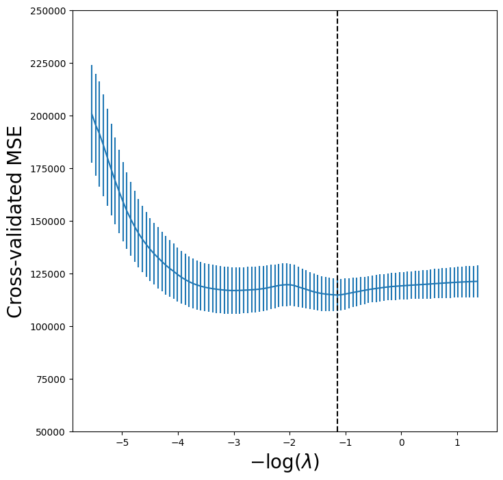
Let’s produce a plot again of the cross-validation error to see that it is similar to using skm.GridSearchCV.

tuned_ridge = pipeCV.named_steps['ridge']
ridgeCV_fig, ax = subplots(figsize=(8,8))
ax.errorbar(-np.log(lambdas),
            tuned_ridge.mse_path_.mean(1),
            yerr=tuned_ridge.mse_path_.std(1) / np.sqrt(K))
ax.axvline(-np.log(tuned_ridge.alpha_), c='k', ls='--')
ax.set_ylim([50000,250000])
ax.set_xlabel('$-\log(\lambda)$', fontsize=20)
ax.set_ylabel('Cross-validated MSE', fontsize=20);

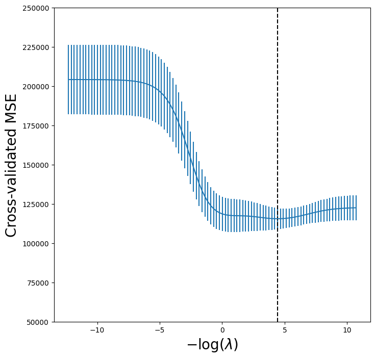
We see that the value of \(\lambda\) that results in the smallest cross-validation error is 1.19e-02, available as the value tuned_ridge.alpha_. What is the test MSE associated with this value of \(\lambda\)?

np.min(tuned_ridge.mse_path_.mean(1))

115526.70630987729

This represents a further improvement over the test MSE that we got using \(\lambda=4\). Finally, tuned_ridge.coef_ has the coefficients fit on the entire data set at this value of \(\lambda\).

tuned_ridge.coef_

array([-222.80877051,  238.77246614,    3.21103754,   -2.93050845,
          3.64888723,  108.90953869,  -50.81896152, -105.15731984,
        122.00714801,   57.1859509 ,  210.35170348,  118.05683748,
       -150.21959435,   30.36634231,  -61.62459095,   77.73832472,
         40.07350744,  -25.02151514,  -13.68429544])

As expected, none of the coefficients are zero—ridge regression does not perform variable selection!

Evaluating Test Error of Cross-Validated Ridge

Choosing \(\lambda\) using cross-validation provides a single regression estimator, similar to fitting a linear regression model as we saw in Chapter~\ref{Ch3:linreg}. It is therefore reasonable to estimate what its test error is. We run into a problem here in that cross-validation will have touched all of its data in choosing \(\lambda\), hence we have no further data to estimate test error. A compromise is to do an initial split of the data into two disjoint sets: a training set and a test set. We then fit a cross-validation tuned ridge regression on the training set, and evaluate its performance on the test set. We might call this cross-validation nested within the validation set approach. A priori there is no reason to use half of the data for each of the two sets in validation. Below, we use 75% for training and 25% for test, with the estimator being ridge regression tuned using 5-fold cross-validation. This can be achieved in code as follows:

outer_valid = skm.ShuffleSplit(n_splits=1, 
                               test_size=0.25,
                               random_state=1)
inner_cv = skm.KFold(n_splits=5,
                     shuffle=True,
                     random_state=2)
ridgeCV = skl.ElasticNetCV(alphas=lambdas,
                           l1_ratio=0,
                           cv=inner_cv)
pipeCV = Pipeline(steps=[('scaler', scaler),
                         ('ridge', ridgeCV)]);

results = skm.cross_validate(pipeCV, 
                             X,
                             Y,
                             cv=outer_valid,
                             scoring='neg_mean_squared_error')
-results['test_score']

array([132393.84003227])

The Lasso

We saw that ridge regression with a wise choice of \(\lambda\) can outperform least squares as well as the null model on the Hitters data set. We now ask whether the lasso can yield either a more accurate or a more interpretable model than ridge regression. In order to fit a lasso model, we once again use the ElasticNetCV() function; however, this time we use the argument l1_ratio=1. Other than that change, we proceed just as we did in fitting a ridge model.

lassoCV = skl.ElasticNetCV(n_alphas=100, 
                           l1_ratio=1,
                           cv=kfold)
pipeCV = Pipeline(steps=[('scaler', scaler),
                         ('lasso', lassoCV)])
pipeCV.fit(X, Y)
tuned_lasso = pipeCV.named_steps['lasso']
tuned_lasso.alpha_

3.1472370031649866

lambdas, soln_array = skl.Lasso.path(Xs, 
                                    Y,
                                    l1_ratio=1,
                                    n_alphas=100)[:2]
soln_path = pd.DataFrame(soln_array.T,
                         columns=D.columns,
                         index=-np.log(lambdas))

We can see from the coefficient plot of the standardized coefficients that depending on the choice of tuning parameter, some of the coefficients will be exactly equal to zero.

path_fig, ax = subplots(figsize=(8,8))
soln_path.plot(ax=ax, legend=False)
ax.legend(loc='upper left')
ax.set_xlabel('$-\log(\lambda)$', fontsize=20)
ax.set_ylabel('Standardized coefficiients', fontsize=20);

The smallest cross-validated error is lower than the test set MSE of the null model and of least squares, and very similar to the test MSE of 115526.71 of ridge regression (page~pageref{page:MSECVRidge}) with \(\lambda\) chosen by cross-validation.

np.min(tuned_lasso.mse_path_.mean(1))

114690.73118253677

Let’s again produce a plot of the cross-validation error.

lassoCV_fig, ax = subplots(figsize=(8,8))
ax.errorbar(-np.log(tuned_lasso.alphas_),
            tuned_lasso.mse_path_.mean(1),
            yerr=tuned_lasso.mse_path_.std(1) / np.sqrt(K))
ax.axvline(-np.log(tuned_lasso.alpha_), c='k', ls='--')
ax.set_ylim([50000,250000])
ax.set_xlabel('$-\log(\lambda)$', fontsize=20)
ax.set_ylabel('Cross-validated MSE', fontsize=20);

However, the lasso has a substantial advantage over ridge regression in that the resulting coefficient estimates are sparse. Here we see that 6 of the 19 coefficient estimates are exactly zero. So the lasso model with \(\lambda\) chosen by cross-validation contains only 13 variables.

tuned_lasso.coef_

array([-210.01008773,  243.4550306 ,    0.        ,    0.        ,
          0.        ,   97.69397357,  -41.52283116,   -0.        ,
          0.        ,   39.62298193,  205.75273856,  124.55456561,
       -126.29986768,   15.70262427,  -59.50157967,   75.24590036,
         21.62698014,  -12.04423675,   -0.        ])

As in ridge regression, we could evaluate the test error of cross-validated lasso by first splitting into test and training sets and internally running cross-validation on the training set. We leave this as an exercise.

PCR and PLS Regression

Principal Components Regression

Principal components regression (PCR) can be performed using PCA() from the sklearn.decomposition module. We now apply PCR to the Hitters data, in order to predict Salary. Again, ensure that the missing values have been removed from the data, as described in Section~\ref{Ch6-varselect-lab:lab-1-subset-selection-methods}.

We use LinearRegression() to fit the regression model here. Note that it fits an intercept by default, unlike the OLS() function seen earlier in Section~\ref{Ch6-varselect-lab:lab-1-subset-selection-methods}.

pca = PCA(n_components=2)
linreg = skl.LinearRegression()
pipe = Pipeline([('pca', pca),
                 ('linreg', linreg)])
pipe.fit(X, Y)
pipe.named_steps['linreg'].coef_

array([0.09846131, 0.4758765 ])

When performing PCA, the results vary depending on whether the data has been standardized or not. As in the earlier examples, this can be accomplished by including an additional step in the pipeline.

pipe = Pipeline([('scaler', scaler), 
                 ('pca', pca),
                 ('linreg', linreg)])
pipe.fit(X, Y)
pipe.named_steps['linreg'].coef_

array([106.36859204,  21.60350456])

We can of course use CV to choose the number of components, by using skm.GridSearchCV, in this case fixing the parameters to vary the n_components.

param_grid = {'pca__n_components': range(1, 20)}
grid = skm.GridSearchCV(pipe,
                        param_grid,
                        cv=kfold,
                        scoring='neg_mean_squared_error')
grid.fit(X, Y)

GridSearchCV(cv=KFold(n_splits=5, random_state=0, shuffle=True),
             estimator=Pipeline(steps=[('scaler', StandardScaler()),
                                       ('pca', PCA(n_components=2)),
                                       ('linreg', LinearRegression())]),
             param_grid={'pca__n_components': range(1, 20)},
             scoring='neg_mean_squared_error')

In a Jupyter environment, please rerun this cell to show the HTML representation or trust the notebook.
On GitHub, the HTML representation is unable to render, please try loading this page with nbviewer.org.

Let’s plot the results as we have for other methods.

pcr_fig, ax = subplots(figsize=(8,8))
n_comp = param_grid['pca__n_components']
ax.errorbar(n_comp,
            -grid.cv_results_['mean_test_score'],
            grid.cv_results_['std_test_score'] / np.sqrt(K))
ax.set_ylabel('Cross-validated MSE', fontsize=20)
ax.set_xlabel('# principal components', fontsize=20)
ax.set_xticks(n_comp[::2])
ax.set_ylim([50000,250000]);

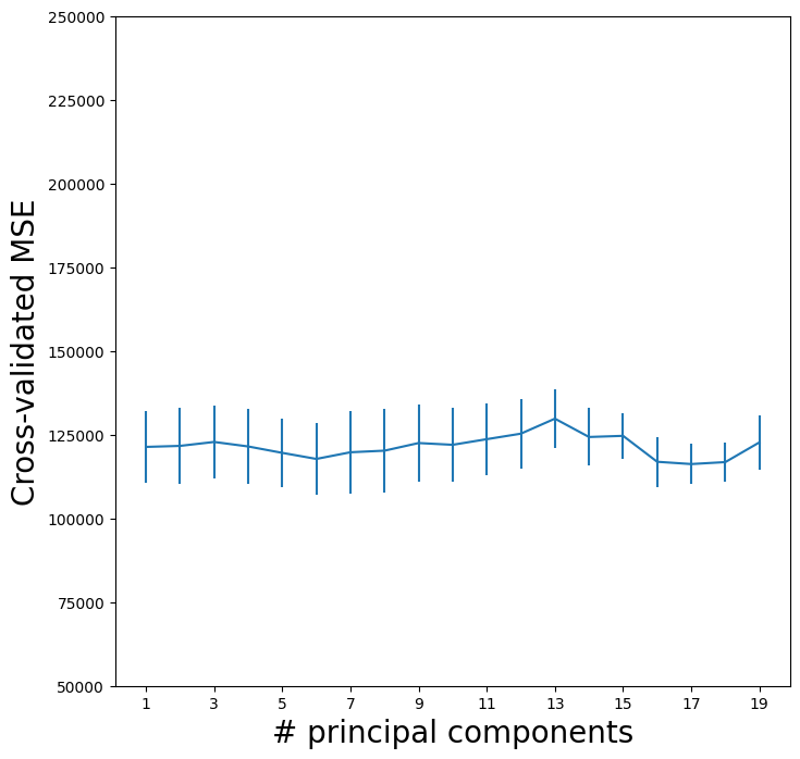
We see that the smallest cross-validation error occurs when 17 components are used. However, from the plot we also see that the cross-validation error is roughly the same when only one component is included in the model. This suggests that a model that uses just a small number of components might suffice.

The CV score is provided for each possible number of components from 1 to 19 inclusive. The PCA() method complains if we try to fit an intercept only with n_components=0 so we also compute the MSE for just the null model with these splits.

Xn = np.zeros((X.shape[0], 1))
cv_null = skm.cross_validate(linreg,
                             Xn,
                             Y,
                             cv=kfold,
                             scoring='neg_mean_squared_error')
-cv_null['test_score'].mean()

204139.30692994667

The explained_variance_ratio_ attribute of our PCA object provides the percentage of variance explained in the predictors and in the response using different numbers of components. This concept is discussed in greater detail in Section~\ref{Ch10:sec:pca}.

pipe.named_steps['pca'].explained_variance_ratio_

array([0.3831424 , 0.21841076])

Briefly, we can think of this as the amount of information about the predictors that is captured using \(M\) principal components. For example, setting \(M=1\) only captures 38.31% of the variance, while \(M=2\) captures an additional 21.84%, for a total of 60.15% of the variance. By \(M=6\) it increases to 88.63%. Beyond this the increments continue to diminish, until we use all \(M=p=19\) components, which captures all 100% of the variance.

Partial Least Squares

Partial least squares (PLS) is implemented in the PLSRegression() function.

pls = PLSRegression(n_components=2, 
                    scale=True)
pls.fit(X, Y)

PLSRegression()

In a Jupyter environment, please rerun this cell to show the HTML representation or trust the notebook.
On GitHub, the HTML representation is unable to render, please try loading this page with nbviewer.org.

As was the case in PCR, we will want to use CV to choose the number of components.

param_grid = {'n_components':range(1, 20)}
grid = skm.GridSearchCV(pls,
                        param_grid,
                        cv=kfold,
                        scoring='neg_mean_squared_error')
grid.fit(X, Y)

GridSearchCV(cv=KFold(n_splits=5, random_state=0, shuffle=True),
             estimator=PLSRegression(),
             param_grid={'n_components': range(1, 20)},
             scoring='neg_mean_squared_error')

In a Jupyter environment, please rerun this cell to show the HTML representation or trust the notebook.
On GitHub, the HTML representation is unable to render, please try loading this page with nbviewer.org.

As for our other methods, we plot the MSE.

pls_fig, ax = subplots(figsize=(8,8))
n_comp = param_grid['n_components']
ax.errorbar(n_comp,
            -grid.cv_results_['mean_test_score'],
            grid.cv_results_['std_test_score'] / np.sqrt(K))
ax.set_ylabel('Cross-validated MSE', fontsize=20)
ax.set_xlabel('# principal components', fontsize=20)
ax.set_xticks(n_comp[::2])
ax.set_ylim([50000,250000]);

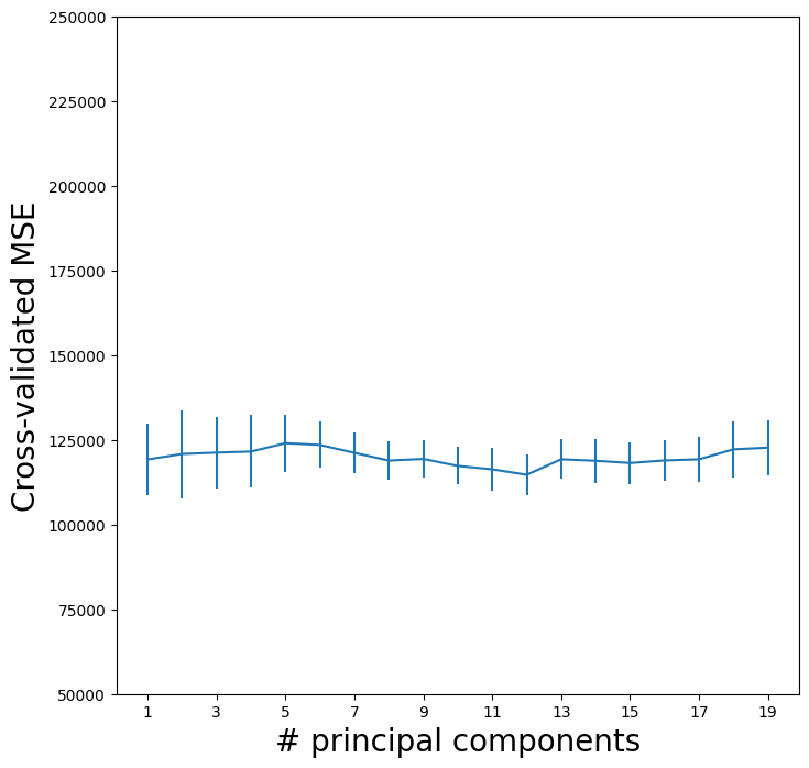
CV error is minimized at 12, though there is little noticable difference between this point and a much lower number like 2 or 3 components.